ELI5: FlashAttention
The goal of this blog post is to explain flash attention in such a way that hopefully anyone who already understands attention will ask themselves:
“Why didn’t I think of this before?” followed by “It’s so easy”.
We’ll start from the first principles. We’ll first understand how the standard/vanilla attention is implemented and then we’ll address the inefficiencies one by one — as if we were to independently discover flash attention ourselves.
Also, my sub-goal is to demystify some of the lingo from the compilers folks’ community: kernel, kernel fusion, materialization, etc.
Note: I won’t be explaining attention itself, for that refer to Jay Alammar’s awesome blog or my implementation of the original transformer paper.
Without further ado let’s start by breaking down the paper title:
“FlashAttention: Fast and Memory-Efficient Exact Attention with IO-Awareness”
The takeaway is that FlashAttention is:
- Fast — excerpt from the paper: “We train BERT-large (seq. length 512) 15% faster than the training speed record in MLPerf 1.1, GPT2 (seq. length 1K) 3x faster than baseline implementations from HuggingFace and Megatron-LM, and long-range arena (seq. length 1K-4K) 2.4x faster than baselines.”
- Memory-efficient — compared to vanilla attention, which is quadratic in sequence length, O(N²), this method is sub-quadratic/linear in N (O(N)). We’ll see later why & how.
- Exact — meaning it’s not an approximation of the attention mechanism (like e.g. sparse, or low-rank matrix approximation methods) — its outputs are the same as in the “vanilla” attention mechanism.
- IO aware — compared to vanilla attention, flash attention is sentient.

Joking :) — it just means that it does not treat the underlying hardware as a black box. Instead, it leverages the knowledge of the memory hierarchy of the underlying hardware (e.g. GPUs, but other AI accelerators should work as well, I’ll be using GPUs as the running example).
Let’s expand on this IO awareness part a bit more. “IO” is the reason more FLOPS doesn’t necessarily translate into longer wall-clock time (maybe somewhat counterintuitively, but obvious if you know how the HW works).
Relevant excerpt from the paper:
“Although these [approximate] methods reduce the compute requirements to linear or near-linear in sequence length, many of them do not display wall-clock speedup against standard attention and have not gained wide adoption. One main reason is that they focus on FLOP reduction (which may not correlate with wall-clock speed) and tend to ignore overheads from memory access (IO).”
What’s the trick?
It’s the hardware:

Over the years GPUs have been adding compute capacity (FLOPS) at a faster pace than increasing the memory throughput (TB/s).
It doesn’t matter if you can compute at exaFLOPS speeds if there is no data to be processed. These 2 need to be closely aligned, and since the hardware lost that balance we have to make our software compensate for it.
Hence “IO-aware”.
Depending on this ratio between computation and memory accesses, operations can be classified as either:
- compute-bound (example: matrix multiplication)
- OR memory-bound (examples: elementwise ops (activation, dropout, masking), reduction ops (softmax, layer norm, sum, etc.)…)
Note on the terminology: this ratio is commonly measured by the arithmetic intensity, which is the number of arithmetic operations per byte of memory access.
Note 2: I strongly recommend reading Horace’s blog post https://horace.io/brrr_intro.html — it’ll help further clarify differences between being compute/memory/overhead-bound.
It turns out attention is (on current AI accelerators) memory-bound.
Why?
Because it “mostly consists of elementwise ops” or more accurately the arithmetic density of attention is not very high.
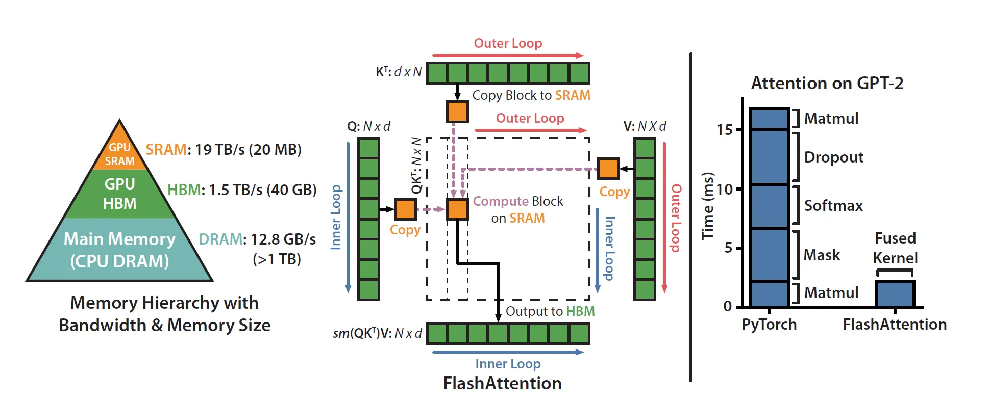
Let’s zoom in on this diagram from the paper:

You can see on the left bar, that masking, softmax & dropout are the ops that are taking the bulk of the time and not matrix multiplication (even though bulk of the FLOPS is in matmul).
But all is not lost. Memory is not a monolithic artifact, it’s hierarchical in its nature and the general rule is: the faster the memory, the more expensive it is, and the smaller its capacity.
Let’s zoom in on this part of the diagram:

Being “IO-aware” in practice boils down to exploiting the fact that SRAM is so much faster than HBM (“high bandwidth memory” — unfortunate name) by making sure to reduce the communication between the two.
To make things a bit less abstract here is a concrete example:
A100 GPU has 40–80GB of high bandwidth memory (HBM, the thing that gives you lovely CUDA OOMs) with a bandwidth of 1.5–2.0 TB/s and 192KB of on-chip SRAM per each of 108 streaming multiprocessors with bandwidth estimated around 19TB/s.
Similar ratios still hold for H100 and other accelerators.
Now, let’s see the computations behind the standard attention implementation:

You can see how the standard implementation shows the utmost disrespect for the way HW operates. It’s basically treating HBM load/store ops as 0 cost (it’s not “IO-aware”).
Let’s now think from the first principles about how we could make this implementation more efficient (time & memory-wise).
The lowest hanging fruit is to remove redundant HBM reads/writes.
Why write S back to HBM only to (re)load it again in order to compute the softmax? Let’s keep it in SRAM instead, perform all of the intermediate steps, and only then write the final result back to HBM.
This is what compilers folks refer to as “kernel fusion”, one of the most important low-level optimizations in deep learning:

No, not that one, but simply this:

A kernel is basically a fancy way of saying “a GPU operation”.
Fusion means you’re fusing/combining multiple ops together.
So, you are loading from the HBM only once, you execute the fused op, and only then write the results back. By doing this you reduce the communication overhead.
On a side note I honestly think people should stop naming concepts with words just because they sound cool. Kernel is the most overloaded word (2nd only to maybe “model”) in the computer science world. It can mean anything: Linux kernel (core software components of Linux OS), neural tangent kernel, SVM kernel, GPU operation, etc. It’s the HIV Aladeen of the CS world. 😂
One final piece of terminology you’ll find floating around is “materialization”. It refers to the fact that in the above standard attention implementation, we’ve allocated full NxN matrices (S, P). We’ll soon see that that’s the bottleneck flash attention directly tackles reducing the memory complexity from O(N²) to O(N).
Now that the complete background context is set, let’s now dig deeper into the flash attention algorithm.
Flash attention basically boils down to 2 main ideas:
- Tiling (used during both forward & backward passes) — basically chunking the NxN softmax/scores matrix into blocks.
2. Recomputation (used in the backward pass only — if you’re familiar with activation/gradient checkpointing, this will be trivial to understand)
That’s it.
Here is the algorithm:

My job here is done. Hope you enjoyed this blog post, subscribe for more content in the future! 🚀
Just kidding.
Let’s understand a couple more ideas that are needed to get the tiling to work, and then I’ll explain the algo line by line.
FlashAttention algorithm
The main hurdle in getting the tiling approach to work is softmax. In particular, the fact that softmax couples all of the score columns together. Here is how we compute the i-th output of a softmax.

You see that denominator?
That’s the issue.
To compute how much a particular i-th token from the input sequence pays attention to other tokens in the sequence you’d need to have all of those scores readily available (denoted here by z_j) in SRAM.
But let me remind you: SRAM is severely limited in its capacity. You can’t just load the whole thing. N (sequence length) can be 1000 or even 100.000 tokens. So N² explodes fairly quickly.
So here’s the trick, we can actually chop the softmax computation down into smaller blocks and still end up with precisely the same result.
Here are the main formulas:

We can grab only the first B scores (x_1 through x_B) and compute the softmax for them.
These numbers are, at least for now, incorrect. But bear with me, through iterations, we’ll “converge” to a correct result.
Note: you can ignore the m(x) part, at least for now while we’re still in Plato’s world of ideas. Its purpose is solely to avoid numerical instabilities. On some hypothetical hardware from the future that’s more precise (e.g. we represent our data using more bits) this would not be needed. m(x) does not change the final result in any way.
Note: also check out the original papers that introduced the online softmax: https://arxiv.org/abs/1805.02867
https://arxiv.org/abs/2112.05682
Now the trick is that we can combine those per-block partial softmax numbers in a smart way such that the final result is actually correct. Here is the main idea:

So basically, in order to compute the softmax for the scores belonging to the first 2 blocks (of size B), you have to keep track of 2 statistics for each of the blocks: m(x) (maximum score) and l(x) (sum of exp scores).
And then you can seamlessly fuse them together using the normalizing coefficients.
Note: if you do some super basic algebra you’ll easily convince yourself that coefficients make sense. By expanding the f(x) and l(x) terms and multiplying with e^x some terms will simply cancel each other out, that’s the basic manipulation.
This logic continues recursively all the way up to the last, (N/B)-th, block, at which point you have the N-dimensional correct softmax output!
Ok, we now have all of the ingredients we need in order to understand the forward pass of the flash attention algorithm.
Note: the algo below assumes we have a batch of size 1 (i.e. single sequence) and a single attention head, we’ll easily scale it up later (by simply parallelizing across GPU’s streaming multiprocessors — more on that later). Also we ignore dropout & masking for the time being, trivial to add it later.

Let’s now break it down step by step!
Step 0: HBM’s capacity is measured in GBs (e.g. RTX 3090 has 24 GBs of VRAM/HBM, A100 has 40–80 GB, etc.) so allocating Q, K, and V is not an issue.
Step 1: Let’s compute the row/column block sizes. Why ceil(M/4d)? Because query, key, and value vectors are d-dimensional, and, we also need to combine them into the output d-dimensional vector. So this size basically allows us to max out SRAM capacity with q, k, v, and o vectors.
Toy example: assume M = 1000, d = 5. In this example, the block size is (1000/4*5) = 50. So in this example, we would load blocks of 50 q, k, v, o vectors at a time, to make sure we’re reducing the number of reads/writes between HBM/SRAM.
Worth keeping this image in your mind (it will make more sense soon):

As for B_r, I’m not exactly sure why do they perform a min op with d? If anyone knows feel free to leave a comment!
Step 2:

We initialize the output matrix O with all 0s. It’ll act as an accumulator hence that init value. Similarly for l (remember: its purpose is to hold the cumulative denominator for the softmax - the sum of exp scores). m (that holds row-wise maximum scores) is initialized with -inf because we’ll be doing a max operator over it so whatever the first block’s max is — it’ll certainly be larger than -inf — hence this is the natural init value.
Step 3:

We split the Q, K, and V into blocks using the block sizes from Step 1. See also the diagram above.
Step 4:

Similarly split O, l, m into blocks (same block size as Q).
Step 5:

Let’s start looping across the columns i.e. across key/value vectors (outer loop in the diagram above).
Step 6:

Let’s load the K_j and V_j blocks from HBM to SRAM. Remember because of the way we constructed the block sizes we still have 50% of the SRAM unoccupied at this point in time (dedicated to Q and O).

Step 7:

Start the inner loop across the rows i.e. across query vectors (again, see the diagram).
Step 8:

Load Q_i (B_r x d) and O_i (B_r x d) blocks, as well as l_i (B_r) & m_i (B_r) into SRAM.
How do l_i & m_i fit into the SRAM (including all of the intermediate variables) when we computed block size in such a way that we only have enough space for K_j, V_j, Q_i & O_i? I think the answer is: registers (see this CUDA video series to get some intuition on GPU memory hierarchy). But I might be wrong, someone who’s actually implemented this in CUDA please correct me. 🙏 I’m sure I’m missing out on important implementation details by just analyzing the pseudo-algorithm.
Step 9:

Compute the dot product between Q_i (B_r x d) and K_j transposed (d x B_c) to get the scores (B_r x B_c). As you can see we don’t have the whole NxN S (scores) matrix “materialized”. Only a fraction of it (S_i_j)!
Toy example: assuming the outer loop index is j (j=3), inner loop index is i (i=2), N is 25 and the block size is 5 this is what we just computed (assuming 1-based indexing):

Basically the attention scores for tokens 6–10 with tokens 11–15 of our input sequence. But, importantly, these are exact scores, they’ll never change (as opposed to softmax results that will gradually get refined).
Step 10:

Compute m~_i_j, l~_i_j, and P~_i_j using the scores computed in the previous step. It’s trivial.
m~_i_j is computed row-wise, find the max element for each of the above rows.
We get P~_i_j by applying elementwise ops:
- Normalization — take the row max and subtract it from row scores
- Exp
l~_i_j is simply a row-wise sum of the matrix P.
Step 11:

Compute m_new_i and l_new_i. Again fairly simple, let’s reuse the diagram from above:

m_i contains row-wise maximums for all of the blocks that came before (j=1 & j=2, colored in green). m~_i_j contains the row-wise maximums for the current block (colored in yellow). To get the m_new_i we just have to apply a max between m~_i_j & m_i. Similarly for l_new_i (it additionally requires multiplying by coefficients as we saw previously in formula 2).
Step 12 (the most important step):

This is the hardest part of the algorithm but still not that complicated, esp. once you internalize the formulas 1 & 2 for partial softmax computation.

Let’s break down the diag(l) part first.
It basically just allows us to do row-wise scalar multiplication in a matrix form. If you have a list of scalars s (N) and a matrix A (NxN), if you do diag(s)*A you’re basically doing elementwise multiplication of rows of A with those scalars.
Next up notice the similarity between step 12 and formula 1 (pasting it here again for convenience):

So what the 1st term of step 12 does (underlined in green) is it updates the current softmax estimate for the blocks before the current block in the same row of blocks. In case j=1 (that is the first block in this row) the 1st term will be 0 and we’ll just end up with the 2nd term.
The multiplication of the 1st term by diag(l_i) is there to cancel the division by that same constant from the previous iteration (this constant is hidden inside of O_i).
The 2nd term of the expression (underlined in yellow) doesn’t require this canceling of terms because as you can see we’re directly multiplying the P~_i_j matrix with the block of V vectors (V_j).
The e^x terms are there to modify the matrix P~_i_j & O_i by canceling out the m from the previous iteration and instead updating it with the latest estimate (m_new_i) that contains the row-wise max so far.
The easiest way to convince yourself this makes sense is to just simulate a couple of iterations yourself — in case you still didn’t quite get it.
It literally takes 5 minutes. Here is my step-by-step analysis (hope it helps!):


Recall: this is just a current estimate of the final O_i. Only after we iterated through all of the red blocks in the diagram above will we end up having the exact result. And that’s it!
Step 13:

Write the newest cumulative statistics (l_i & m_i) back to HBM. Notice these are of dimension B_r.
Steps 14, 15, 16:

Once the nested for loop is over, O (Nxd) will contain the final result: attention-weighted value vectors for each of the input tokens!
That’s it guys. That’s the forward pass of the flash attention!
This algorithm can easily be extended to “block-sparse FlashAttention”, a sparse attention algorithm that is 2–4 faster than even FlashAttention, scaling up to a sequence length of 64k! The idea is we use a block form mask matrix and we simply skip certain loads/stores from the above nested for loop and by doing so we can save proportionally to the sparsity coefficient.

Now let’s briefly touch on the complexity.
Complexity analysis
Space: We’ve allocated Q, K, V, O (Nxd), l & m (N) in HBM. That’s 4*N*d + 2*N. Dropping the constants (big O stuff), and knowing that d is also a constant and usually much smaller than N (e.g. usually d={32, 64, 128}, N={1024, …, 100k}) we get O(N) for space. Big win! That helps us scale transformers to 64k sequence lengths “easily” (add to that a couple of other “tricks” like ALiBi which I’ll cover in one of the follow-up blog posts).
Time: we won’t strictly do a time complexity analysis, instead we’ll use a good proxy: the number of HBM accesses.
Here is an excerpt from the paper:

How do they get to that number? Well, let’s analyze the nested for loop:
- Our block size is M/4d. This means that the vectors are split into N/(M/4d) blocks.
- Raise that to the power of 2 (because we’re looping across row/column blocks) and we get O(N² d² / M²)
- Now here I have M² and they only have M¹ — my hypothesis is that we probably need M/4d memory accesses inside of the loop to actually fetch all the vectors, i.e. we can’t fetch the whole block all at once. That would explain the missing M? (d can be ignored as a constant in big O).
If we were to do a big O analysis that could lead us to think this is not much better than standard attention, but for typical numbers, this leads to up to 9x fewer accesses (as per the excerpt above).
And that’s it, you now (hopefully) understand the flash attention!
Let’s wrap it up by closing the gap with the real world. So far we were analyzing the pseudo algorithm focusing on a single attention head assuming a batch size of 1. And we also glossed over the backward pass.
batch_size > 1, num_heads > 1, backward pass
Let’s start with the low-hanging fruit. Extending the implementation we saw to support batch_size > 1 and the num_heads > 1 is actually not that hard.
So far the algorithm we saw is basically handled by a single thread block (CUDA programming lingo). This thread block is executed on a single streaming multiprocessor (SM) (e.g. there are 108 of these on A100). To parallelize our computation we just run batch_size * num_heads threadblocks in parallel on different SMs. The closer that number is to the number of available SMs on the system the higher the utilization will be (ideally a multiple as each SM can run multiple thread blocks).
What happens when that number is bigger than the number of available SMs? I’m not sure but I assume there is a queue that keeps track of the waiting kernels (update: apparently the CUDA runtime takes care of that and it is using some sort of queues to implement that logic).
Next up let’s briefly address the backward pass.
The backward pass relies on the same set of concepts + recomputation.
To demonstrate the concept of recomputation I’ll use the example of “activation/gradient checkpointing” method.
We know that we need to have the activations computed during the forward pass readily available during the backward pass in order to compute the gradients w.r.t. our loss function.
The trick here is to not store them during the fwd pass (as they have a huge memory footprint), but instead, recompute them de novo during the backward pass. There is a built-in tradeoff here: we’re slowing down the backward pass in order to reduce the memory footprint.
Note: This tradeoff is a spectrum, e.g. you can store the activations every n layers, and then when computing the activations for the i-th layer you don’t have to start from the input but instead from the closest stored activations.
The same concept of recomputation is re-used here — but with a twist! Luckily for the flash attention, we don’t have to sacrifice neither runtime nor memory!
By storing the output O (Nxd) and the softmax normalization statistics (N) we can recompute the attention matrices S (NxN) and P (NxN) in the backward pass directly from blocks of Q, K, and V (Nxd) in SRAM! Thus keeping the memory at O(N). I encourage you to read the paper if you’re curious about the details, but I assure you, you’re equipped with all of the tools you need to understand it now.
Lastly, let’s see some of the issues one could expect implementing flash attention.
The real world is…messy
The same thing that gives flash attention its power is the root cause of its issues. Let’s see this excerpt from the paper:
“Our current approach to building IO-aware implementations of attention requires writing a new CUDA kernel for each new attention implementation. This requires writing the attention algorithm in a considerably lower-level language than PyTorch, and requires significant engineering effort. Implementations may also not be transferrable across GPU architectures. These limitations suggest the need for a method that supports writing attention algorithms in a high-level language (e.g., PyTorch), and compiling to IO-aware implementations in CUDA…”
As a consequence, the original flash attention supported only a subset of GPUs. For example, V100 is not supported. See this issue on their GitHub:

Note: here is one more relevant issue: https://github.com/HazyResearch/flash-attention/issues/190
To make this issue a bit more visceral, here is the actual CUDA code from the original implementation:

As you can see, writing CUDA is…messy. Additionally — this is a research codebase which doesn’t help, but even if it wasn’t for someone coming from an ML research background, who is only comfortable with Python this is (potentially) a deal breaker.
This is where projects like OpenAI’s Triton could be game changers (see their FlashAttention implementation). Triton is basically a DSL (domain-specific language) between CUDA & other DSLs (e.g. TVM) in its level of abstraction. You can write Python code that’s super optimized (once compiled) instead of having to deal directly with CUDA. That very same Python code could then be deployed on an arbitrary accelerator (that responsibility lies on Triton devs and HW manufacturers).
Triton has recently been integrated with PyTorch 2.0 so definitely keep an eye out for this project! Shout out to Philippe Tillet who started building Triton during his PhD and later became a part of OpenAI.
Finally, it’s worth mentioning that for certain use cases, you might still prefer other methods. E.g. for sequence lengths beyond 1K, some approximate attention methods (e.g., Linformer) start to become faster. But ultimately, to the best of my understanding, the block-sparse implementation of the flash attention outperforms all other methods.
Outro
You might ask yourself: why didn’t anyone invent FlashAttention before? Given how crucial this piece of computation is to all modern ML workloads. Given how many engineering hours are spent, across different tech organizations, trying to squeeze the last ounce of performance out of these systems. Why did a Stanford student (shout out to Tri Dao for the amazing work!) come up with this and not e.g. NVIDIA engineers?
There is a couple of possible explanations that I can see:
- FlashAttention is, as far as I can tell, easier/only possible to implement on the latest GPUs (hence V100 is not supported in the original codebase). Couple this with the phenomenon that oftentimes “outsiders” are those who see the problems with beginner’s eyes and tackle issues from the first principles and we get to the possible explanation.
- Ultimately I really like Nat Friedman’s perspective on the efficiency of the world:

Finally, let me wrap up with some food for thought:
Given how much it costs to train these models (see this blog from MosaicML for the most optimistic estimates) being able to shave off 15% from BERT-large training, or speed up GPT training 2/3x has such a tremendous economic impact when considering all of the current, and future, model trainings at a global scale.
Imagine if we lived in a world where Y (value captured) was actually correlated with X (value produced). The author would be a trillionaire over the next few years. :)
Alas, researchers rarely capture that value, for better or worse (imagine if Pythagoras patented his theorem :P). Yet people who oftentimes just repackage stuff are those who capture most of the value. Going on a complete tangent here, until next time! ;)
Further resources
- Flashier Attention blog — https://www.adept.ai/blog/flashier-attention -> They show how to further optimize flash attention for highly distributed settings where batch sizes become super small (pipeline parallelism) and sequence length super long.
- Tri Dao’s talk: FlashAttention — Tri Dao | Stanford MLSys #67
- Tri Dao’s talk: MedAI #54: FlashAttention: Fast and Memory-Efficient Exact Attention with IO-Awareness | Tri Dao
- Paper: FlashAttention: Fast and Memory-Efficient Exact Attention with IO-Awareness
Acknowledgments
Thanks to Tri Dao, Horace He, and Amrit Sahu for reading earlier drafts of this blog post and providing feedback!
BibTeX Citation
@article{gordiceli5flashattention,
  author={Aleksa Gordic},
  title={ELI5: FlashAttention},
  year={2023},
  url={https://gordicaleksa.medium.com/eli5-flash-attention-5c44017022ad},
}
Connect with me
Last but not least feel free to drop me a message or:
- Connect and reach out on LinkedIn and/or Twitter
- Subscribe to my YouTube channel for more ML
- Follow me on Medium and GitHub
- Subscribe to my monthly AI newsletter and join the Discord community!
And if you find the content I create useful consider becoming a Patreon!
Much love ❤️